Robotics: Science and Systems · 2026

RSS 2026 Outstanding Paper Award Finalist RSS 2026 Outstanding Student Paper Award Finalist

Realizing Robotic Swimming with
Unified Fluid Robot Multiphysics

Jeong Hun Lee1,†· Junzhe Hu1,†· Sofia Kwok1· Carmel Majidi1· Zachary Manchester1,2

¹ Carnegie Mellon University · ² Massachusetts Institute of Technology

^† Equal contribution

Time-lapse of an optimized C-start escape maneuver from t = 0 to 3 seconds. Top row: hardware. Middle row: unified multiphysics. Bottom row: particle-based simulator. — Optimized C-start escape maneuver on a multi-link eel robot across *t = 0–3 s*. Hardware (top) is closely tracked by our unified multiphysics simulator (middle), while the particle-based simulator (bottom) fails to complete the intended 90° turn.

00 · ContextWhy unified multiphysics?

Robotic swimming is a genuinely strongly coupled problem: the robot reshapes the surrounding flow, and the resulting pressure and viscous forces immediately change the robot's motion. Treating those two systems as separate simulators connected by an external force can miss the vortex interactions that make fish-like locomotion efficient and agile.

Unified least-action overview showing an articulated robot moving through the surrounding fluid velocity field. — Problem setting. A controlled articulated robot with geometry $\Gamma$ moves through an incompressible Newtonian fluid occupying $\Omega$. The no-slip condition on the shared interface must transmit motion and force consistently in both directions.

One physical model

Fluid and robot equations are derived from one constrained action, so coupling is part of the dynamics rather than a post-processing force.

Multibody-ready coupling

An integral-form immersed boundary constraint remains well-conditioned around adjacent links and overlapping boundary nodes.

End-to-end gradients

Implicit differentiation captures how design or gait parameters alter both robot motion and the surrounding fluid state.

01 · MotivationAbstract

Matching the swimming efficiency and agility of fish has remained an elusive goal in underwater robotics. Such locomotion relies on complex vortex interactions between the robot's body and the surrounding fluid, governed by coupled ordinary and partial differential equations — significantly more difficult than the multi-body dynamics of classical rigid robotic systems.

We present a differentiable framework for simulating strongly coupled fluid-robot multiphysics as a unified optimization problem. The coupled manipulator and incompressible Navier–Stokes equations are derived together from a single Lagrangian using the principle of least action. We employ discrete variational mechanics to derive a stable, well-conditioned, and physically accurate scheme for jointly simulating articulated bodies and the surrounding fluid, and leverage the implicit function theorem to compute derivatives through the fully coupled dynamics.

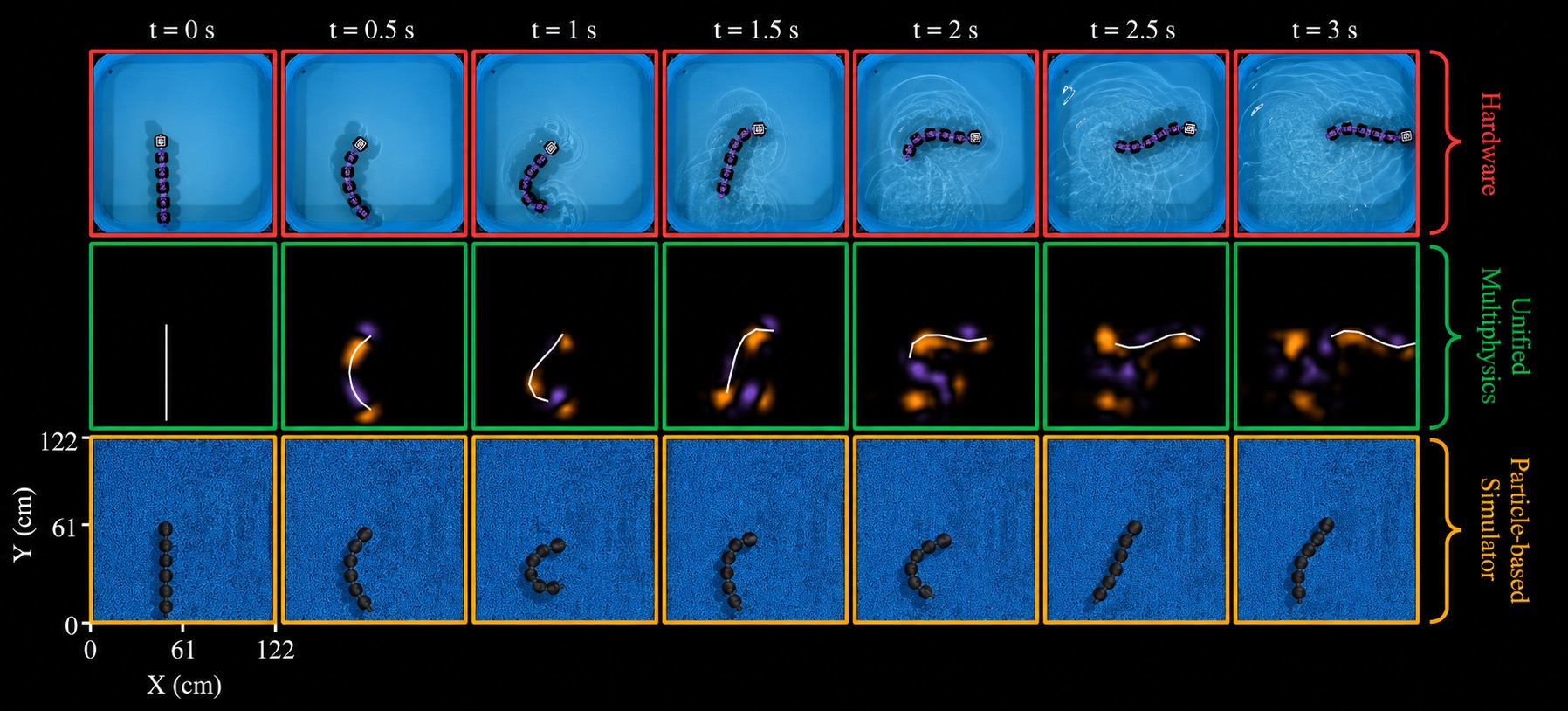
Using this simulator and its gradients, we realize undulating swimming gaits and optimize a highly dynamic C-start escape maneuver for a bioinspired eel robot. We validate both gaits on physical hardware, demonstrating successful sim-to-real transfer.

02 · FormulationMethod

Existing multiphysics simulators time-integrate the fluid and robot equations separately, then couple them through an explicit force term. We instead pose the entire problem as a single least-action optimization: the unified Lagrangian is discretized directly, and the coupling forces emerge as Lagrange multipliers of a no-slip constraint.

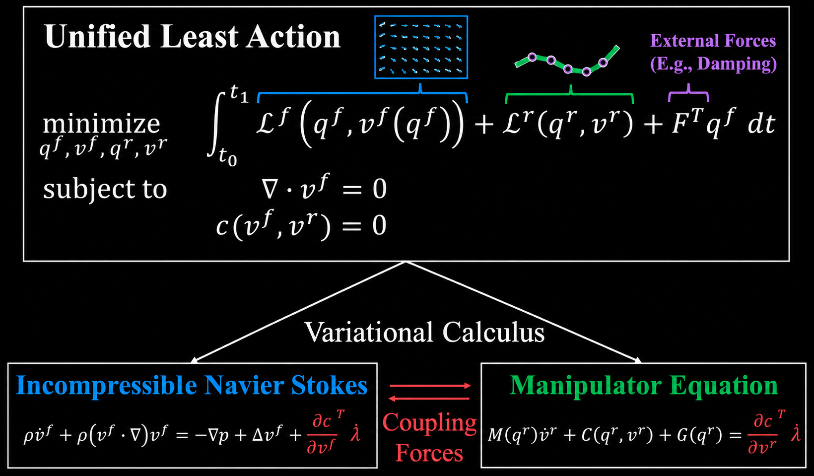
Unified least-action formulation: a single constrained optimization yields the incompressible Navier-Stokes and manipulator equations, coupled through constraint forces. — The unified Lagrangian governing the coupled fluid–robot dynamics. Variational calculus on the combined action recovers the incompressible Navier–Stokes and manipulator equations; the multiphysics coupling stems from a single constraint enforcing no-slip at the fluid–robot interface.

1.From least action to the manipulator equation

For a system with configuration $q(t)\in\R^n$, velocity $v(t)\in\R^m$, kinetic energy $T(v)$, and potential energy $U(q)$, the principle of least action poses the dynamics as a continuous-time optimization problem:

$$\min_{q,\,v}\;\; \int_{t_0}^{t_f} T\!\big(v(t)\big) - U\!\big(q(t)\big)\, dt \quad\text{s.t.}\quad v=\dot{q}.$$ (1)

Introducing a Lagrange multiplier $\lambda$ for the kinematic constraint and writing $L(q,v) = T(v) - U(q)$, the action becomes $\;S(q,v)=\int_{t_0}^{t_f} L(q,v) + \lambda^\top(\dot q - v)\, dt.$ Stationarity yields the Euler–Lagrange equation

$$\frac{d}{dt}\frac{\partial L}{\partial \dot q} - \frac{\partial L}{\partial q} \;=\; 0,$$ (2)

which in robotics is more familiar as the manipulator equation $\;M(q)\ddot q + C(q,\dot q)\dot q + G(q) = 0.$ The least-action principle generalizes to dissipative systems via Lagrange–D'Alembert, to non-trivial kinematics $v=f(q,\dot q)$, and to additional constraints $c(q,v)=0$:

$$\min_{q,\,v}\; \int_{t_0}^{t_f} T(q,v) - U(q) + F(t)^\top q(t)\, dt \;\;\text{s.t.}\;\; v=f(q,\dot q),\;\; c(q,v)=0.$$ (3)

2.A unified Lagrangian for fluid–robot multiphysics

For a rigid multibody robot interacting with an incompressible Newtonian fluid (e.g., water), we define fluid and robot Lagrangians as

$$L^f(q^f,v^f) = \int_\Omega \tfrac{1}{2}\rho\, (v^f)^\top v^f - \rho\, g^\top q^f \, dV$$ (4)

$$L^r(q^r,v^r) = \tfrac{1}{2}(v^r)^\top M^r v^r - M^r g^\top q^r$$ (5)

where $\rho$ is fluid density, $\mu$ its dynamic viscosity, $\Omega$ the fluid domain with boundary $\partial\Omega$, $\Gamma$ the robot geometry with boundary $\partial\Gamma$, and $M^r$ the robot mass matrix. Damping enters via the viscous term $F(t)=\int_\Omega \mu\,\Delta v^f\, dV$. The full multiphysics is then a single constrained optimization over fluid and robot states:

Unified least action

$$\begin{aligned} \min_{q^r,\,v^r,\,q^f,\,v^f}\;\; & \int_{t_0}^{t_f}\! \textcolor{#0090e9}{L^f(q^f,v^f)} + \textcolor{#00ba58}{L^r(q^r,v^r)} + F(t)^\top q^f \, dt \\[2pt] \text{s.t.}\;\; & c_1(v^f)=\dot q^f - v^f(q^f)=0 && \forall\, q^f\in\Omega \\ & c_2(v^f)=\nabla\!\cdot v^f = 0 && \forall\, q^f\in\Omega \\ & c_3(v^f)=v^f - v_{bc}=0 && \forall\, q^f\in\partial\Omega \\ & c_4(v^r)=\dot q^r - v^r=0 && \forall\, q^r \\ & c_5(q^r)=0 && \forall\, q^r \\ & \textcolor{#b268da}{c_6(v^f,v^r)=v^f - {}^bv^r=0} && \forall\, q^f\in\Gamma \end{aligned}$$

(6)

Constraints $c_1\!-\!c_4$ are the standard kinematic and conservation conditions; $c_5$ encodes joint constraints; $c_6$ is the no-slip condition at the fluid-robot interface and is the only coupling between the two physics.

Forming the action $S = \int (L^f + L^r + F^\top q^f + \sum_{i=1}^6 \lambda_i c_i)\, dt$ and taking variations w.r.t. $(q^f,v^f)$ and $(q^r,v^r)$ recovers the coupled incompressible Navier–Stokes and manipulator equations:

$$\rho\!\left(\dot v^f + (v^f\!\cdot\!\nabla) v^f\right) = -\nabla p + \mu\nabla^2 v^f - \rho g \;- \tfrac{\partial c_3}{\partial v^f}^{\!\!\top}\!\dot\lambda_3 \;\textcolor{#b268da}{- \tfrac{\partial c_6}{\partial v^f}^{\!\!\top}\!\dot\lambda_6}$$ (7)

$$\nabla\!\cdot v^f = 0$$ (8)

$$M^r \dot v^r + \rho g = \tfrac{\partial c_5}{\partial q^r}^{\!\!\top}\!\lambda_5 \;\textcolor{#b268da}{-\, \tfrac{\partial c_6}{\partial v^r}^{\!\!\top}\!\dot\lambda_6}, \qquad \dot q^r = v^r$$ (9)

Where the coupling lives

The purple terms in (7) and (9) share the same dual variable $\lambda_6$. The pressure $p \equiv \dot\lambda_2$ is itself the multiplier that enforces $\nabla\!\cdot v^f=0$ — a fact Lagrange noted in his Mécanique analytique. Boundary conditions and the no-slip interface inherit the same constraint-with-dual-variable structure that Allmaras (2005) used for compressible aerodynamics.

3.A variational integrator that handles the temporal lag

Discretizing the action in time is delicate. A midpoint quadrature gives a discrete Lagrangian $L_d(q_k,q_{k+1}) = h\,L\!\left(\tfrac{q_k+q_{k+1}}{2},\,\tfrac{q_{k+1}-q_k}{h}\right)$ in which the velocity $\bv_k$ lives between the configurations $q_k$ and $q_{k+1}$. For pure rigid-body simulation this half-step delay is harmless. For our problem it is not: the fluid is represented as a velocity field $\bv^f$ while the robot pose lives in $q^r$, and the no-slip constraint must couple them at a consistent time.

Midpoint variational integrator showing robot configurations at integer time steps and fluid velocity fields at half time steps, creating a temporal mismatch. — Temporal mismatch in a conventional midpoint variational integrator. Robot configurations $q_k$ are defined at integer time steps, while the fluid velocity $\bar v_k$ is evaluated at the midpoint of each interval. Our formulation integrates the full fluid–robot variational state while enforcing each constraint at the time where its variables naturally live.

Marsden & West (2001) resolve this via the discrete Legendre transform, which is awkward in the presence of constraints. We instead define every constraint at the time step at which its variable naturally lives ($q_k$ for the robot, $\bv_k$ for the fluid), and rewrite the discrete Euler–Lagrange relation directly via the chain rule:

$$D_2 L_d(q_{k-1},q_k) = h\!\left(\tfrac{\partial L}{\partial \bq_k}\!\cdot\!\tfrac{1}{2} + \tfrac{\partial L}{\partial \bv_k}\!\cdot\!\tfrac{1}{h}\right)$$ (10)

$$D_1 L_d(q_k,q_{k+1}) = h\!\left(\tfrac{\partial L}{\partial \bq_{k+1}}\!\cdot\!\tfrac{1}{2} + \tfrac{\partial L}{\partial \bv_{k+1}}\!\cdot\!\big(\!-\!\tfrac{1}{h}\big)\right)$$ (11)

Substituting these back into the discrete Euler–Lagrange equation produces, after some algebra, two coupled update rules — one for the robot, one for the fluid — that are simultaneously solved each time step. With $\bv^r_{k+1}$ and $\bv^f_{k+1}$ as unknowns:

$$\tfrac{1}{2}M^r \bv^r_{k+1} \,-\, h\!\left(\tfrac{\partial c_5}{\partial q^r_k}\right)^{\!\!\top}\!\lambda_{5,k} \,\textcolor{#b268da}{-\, h\!\left(\tfrac{\partial c_6}{\partial \bv^r_k}\right)^{\!\!\top}\!\lambda_{6,k}} = \tfrac{1}{2}M^r \bv^r_k - h M^r g$$ (12)

$$\begin{aligned} \tfrac{1}{2}(M^f - \mu h L)\bv^f_{k+1} &- \tfrac{h}{2} N(\bv^f_{k+1}) + G\, p_k + B\,\lambda_{3,k} \textcolor{#b268da}{- h\!\left(\tfrac{\partial c_6}{\partial \bv^f_k}\right)^{\!\!\top}\!\lambda_{6,k}} \\ &\quad = \tfrac{1}{2}(M^f + \mu h L)\bv^f_k + \tfrac{h}{2}N(\bv^f_k) - h M^f g \end{aligned}$$ (13)

Together with the discrete constraints $G^\top \bv^f_{k+1}=0$ (incompressibility), $B\bv^f_{k+1}=v_{bc}$ (boundary), $\bar E\,\bv^f_{k+1} = {}^b\bv^r(\bv^r_{k+1})$ (no-slip), and $c_5(q^r_{k+1})=0$ (joints), the system forms a sparse nonlinear root-finding problem solved by Newton's method. The resulting scheme is a 2nd-order implicit leap-frog integrator, and derivatives through it are obtained from the implicit function theorem.

Spatial discretization — finite-volume operators

The fluid domain is discretized with a second-order finite-volume scheme yielding the following discrete counterparts of the continuous operators that appear in the Navier–Stokes equations:

$\;\int_\Omega \rho v^f\, dV \mapsto M^f v^f,\quad \int_\Omega \nabla p\, dV \mapsto Gp,\quad \int_\Omega (v^f\!\cdot\!\nabla)v^f\, dV \mapsto N(v^f),\quad \int_\Omega \Delta v^f\, dV \mapsto Lv^f.$

$M^f$ is the lumped fluid mass matrix, $G$ the discrete gradient, $N(\cdot)$ the (nonlinear) convection operator, and $L$ the discrete Laplacian. $B$ extracts cells on $\partial\Omega$.

4.An integral-form immersed boundary for multibody robots

The classical immersed-boundary method enforces no-slip pointwise: $\;\int_\Omega v^f\,\delta(q^f-{}^bq^r)\, d\Omega = {}^bv^r,\;$ discretized as $\;E v^f - {}^bv^r = 0,\;$ with a convolution matrix $E$ built from a smoothed delta. This satisfies no-slip only at a finite set of boundary nodes — allowing fluid penetration when nodes are sparse, and producing redundant, ill-conditioned constraints when nodes from neighboring bodies overlap. Both pathologies are common in articulated robots.

Immersed-boundary coupling between an articulated robot and a fluid grid, comparing the original pointwise no-slip constraint with the proposed integral-form constraint along each body segment. — Multibody immersed-boundary coupling. The original formulation matches fluid and robot velocity only at discrete boundary nodes, which can permit penetration between sparse nodes or become singular when nodes overlap. Integrating the constraint along each body segment produces a weak-form no-slip condition that remains well-conditioned for articulated robots.

We instead integrate the constraint along the whole boundary $\Gamma$:

$$\oint_\Gamma\!\int_\Omega v^f\, \delta\!\big(q^f-{}^bq^r(q^r)\big)\, dV\, dS \;=\; \oint_\Gamma {}^bv^r(q^r,v^r)\, dS$$ (14)

Discretizing with piecewise-linear interpolation along the boundary and integrating the smoothed delta along each segment yields a new convolution matrix $\bar E$:

$$\bar E\, v^f - {}^bv^r(v^r) \;=\; 0$$ (15)

Unlike the pointwise form, $\bar E$ stays well-conditioned when boundary nodes overlap, and the constraint is satisfied between nodes rather than only at them. Differentiating through (15) inside (12)–(13) gives the multibody-friendly coupling we use throughout the paper.

5.Optimizing through fluid–robot gradients

Differentiability turns the simulator into an optimization tool rather than only a rollout engine. Let $x_k=[q^r,\bar v^r,\bar v^f]_k$ collect the full robot and fluid state, let $\beta$ denote gait or design parameters, and let $f(x_{k+1},x_k;\beta)=0$ denote the implicit coupled update. We solve

Gradient-based optimization

$$\begin{aligned} \min_{\beta}\quad & J(x_{1:N}) \\ \text{s.t.}\quad & f(x_{k+1},x_k;\beta)=0. \end{aligned}$$

Applying the implicit function theorem to the entire nonlinear multiphysics solve gives $\partial x_{k+1}/\partial x_k$ and $\partial x_k/\partial\beta$. Backpropagating those sensitivities through time yields $\nabla_\beta J$, including how every parameter changes both the articulated body and the surrounding flow. We use these gradients with box-constrained L-BFGS to optimize the C-start maneuver below.

Why the unified gradient matters

A robot-only derivative would ignore how a parameter changes vortex formation and hydrodynamic loading. Here the sensitivity passes through the same strongly coupled equations used for simulation.

6.Contributions

A unified derivation of strongly coupled fluid-robot multiphysics via the principle of least action.
A new weak formulation of the no-slip boundary constraint at the fluid-robot interface.
A differentiable fluid-robot multiphysics simulator.
Realization of accurate, dynamic robotic swimming on a bioinspired eel robot with validation against real-world hardware.

03 · ExperimentsResults

Experimental setup

We evaluate the simulator in a 122 × 122 cm cavity of initially still water with walled boundary conditions. The eel is represented in maximal coordinates by six 9.8 cm rigid links connected by five revolute joints. Our finite-volume fluid uses 1 cm cells; the Genesis SPH baseline uses equivalently sized particles so both methods are compared at consistent spatial fidelity.

A six-link eel robot inside a 122 by 122 centimeter walled fluid cavity, with maximal-coordinate link poses and joint angles labeled. — Matched simulation environment. The eel swims in a 122 × 122 cm walled cavity of initially still water. Its six 9.8 cm rigid links are represented in maximal coordinates $(x_i,y_i,\theta_i)$ and connected by commanded revolute-joint angles $\bar\theta_i$.

Steady undulatory swimming

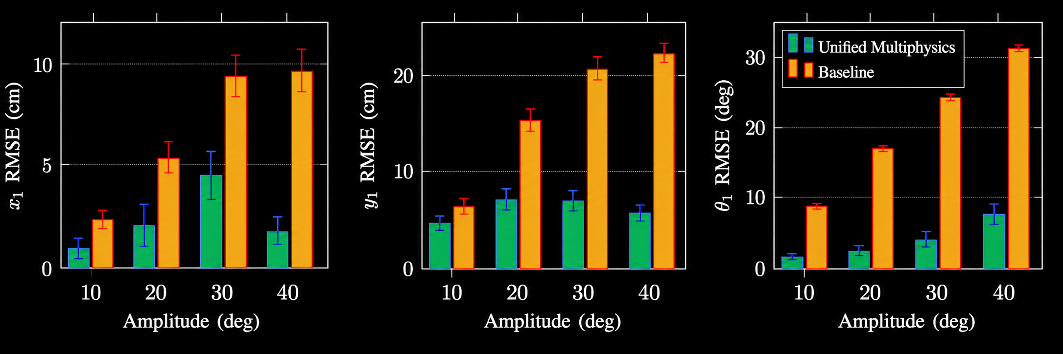
We drive each joint with a phase-shifted sinusoid to produce a traveling wave at 1 Hz with body wavelength $\lambda = L_B$. Across joint amplitudes from 10° to 40° (20 trials each), our method consistently tracks hardware while the SPH baseline drifts — the gap widens with amplitude.

Time-lapse comparison: Hardware, Unified Multiphysics, and Particle-based Simulator at t = 0, 1, 2, 3, 4 seconds. — Time-lapse of forward swimming at 40° amplitude across *t = 0–4 s*. Hardware (top) is closely tracked by our unified multiphysics simulator (middle), while the particle-based baseline (bottom) drifts — the gap widens with amplitude.

Bar charts of head-link RMSE for x1, y1, and theta1 versus undulation amplitude (10, 20, 30, 40 degrees), comparing Unified Multiphysics against the particle-based baseline. — Mean trajectory RMSE of the head-link configuration ($x_1$, $y_1$, $\theta_1$) versus undulation amplitude. Unified multiphysics outperforms the particle-based baseline across all amplitudes, with up to **75%** error reduction at 40°.

Hardware undulatory swimming at 40° amplitude

Our unified multiphysics simulator at 40° amplitude

Genesis particle-based baseline at 40° amplitude

Optimizing a highly dynamic C-start

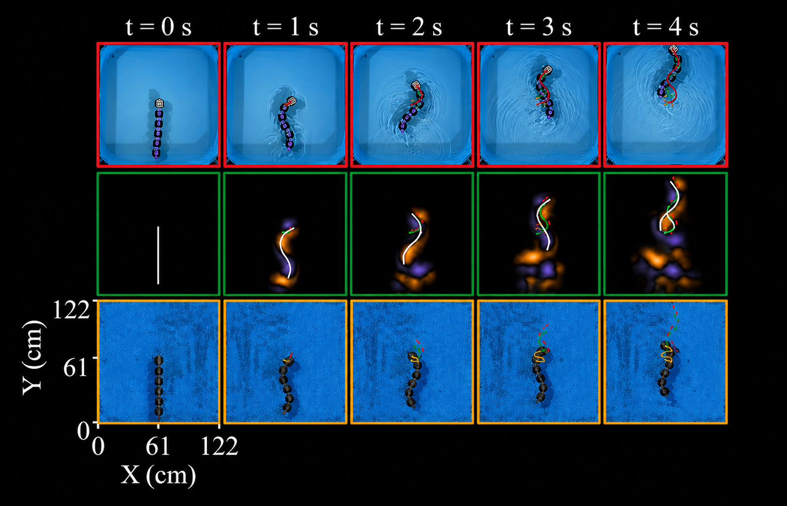
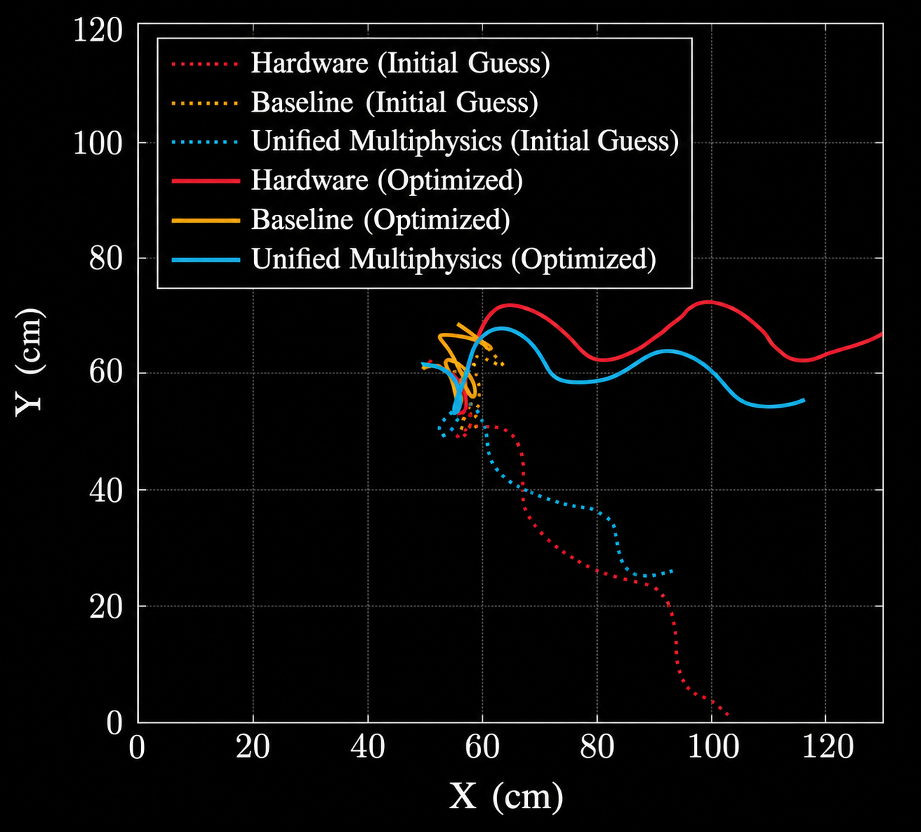
We use the simulator's gradients to optimize a fish-inspired C-start escape maneuver. The robot first curls into a C-shape during a bending phase (0–1 s), then rapidly straightens and launches a traveling wave during the propulsion phase (1–3 s). The terminal objective penalizes error between the final center-of-mass configuration $q_N^{\mathrm{com}}$ and a goal configuration $q_{\mathrm{goal}}$ representing a 90° turn:

$$J(x_N)=\tfrac{1}{2}(q_N^{\mathrm{com}}-q_{\mathrm{goal}})^\top Q(q_N^{\mathrm{com}}-q_{\mathrm{goal}}).$$

We optimize the five bend angles $\bar\theta_{1:5}$, traveling-wave phase $\phi$, and wavelength $\lambda$, while fixing joint amplitude to 25° to avoid the pool wall. Box-constrained L-BFGS uses $10^\circ\!\leq\!\bar\theta_{1:5}\!\leq\!36^\circ$, $-\pi/2\!\leq\!\phi\!\leq\!0$, and $0.5L_B\!\leq\!\lambda\!\leq\!L_B$. Starting from $\bar\theta_{1:5}^{\mathrm{ig}}=10^\circ$, $\phi^{\mathrm{ig}}=-\pi/3$, and $\lambda^{\mathrm{ig}}=0.6L_B$, optimization converges to $[17^\circ,18^\circ,20^\circ,24^\circ,36^\circ]$, $\phi^*=-1.16$, and $\lambda^*=0.57L_B$. The optimized gait executes the desired turn open-loop on hardware; the SPH baseline realizes neither the turn nor the propulsion.

C-start gait parameterization showing a bending phase from zero to one second and a propulsion phase from one to three seconds, with bend angles, phase, and wavelength labeled. — C-start parameterization. During the bending phase (0–1 s), the five joint angles $\bar\theta_{1:5}$ curl the eel into a C-shape. During the propulsion phase (1–3 s), the wave phase $\phi$ and wavelength $\lambda$ govern rapid straightening and a tailward traveling wave that produces reorientation and acceleration.

a.Initial guess (before optimization)

Hardware C-start with the initial (un-optimized) parameters

Our unified multiphysics simulator C-start before optimization

Genesis particle-based baseline C-start before optimization

b.After gradient-based optimization — 90° turn from rest

Our unified multiphysics simulator optimized C-start, 90° turn

Genesis particle-based baseline rolled out with the optimized control trajectory

Computational cost

A 3-second C-start rollout contains 300 steps at 100 Hz. On an M3 Ultra Mac Studio CPU, our implicit unified solve completes the rollout in approximately 261 s. The matched Genesis SPH rollout takes 2727 s on the same CPU and 300 s on an NVIDIA RTX 3070 Ti GPU.

261 s Unified multiphysics
28-core M3 Ultra CPU
0.87 s per step

2727 s Genesis SPH
28-core M3 Ultra CPU
9.09 s per step

300 s Genesis SPH
NVIDIA RTX 3070 Ti GPU
1.00 s per step

04 · PlatformHardware

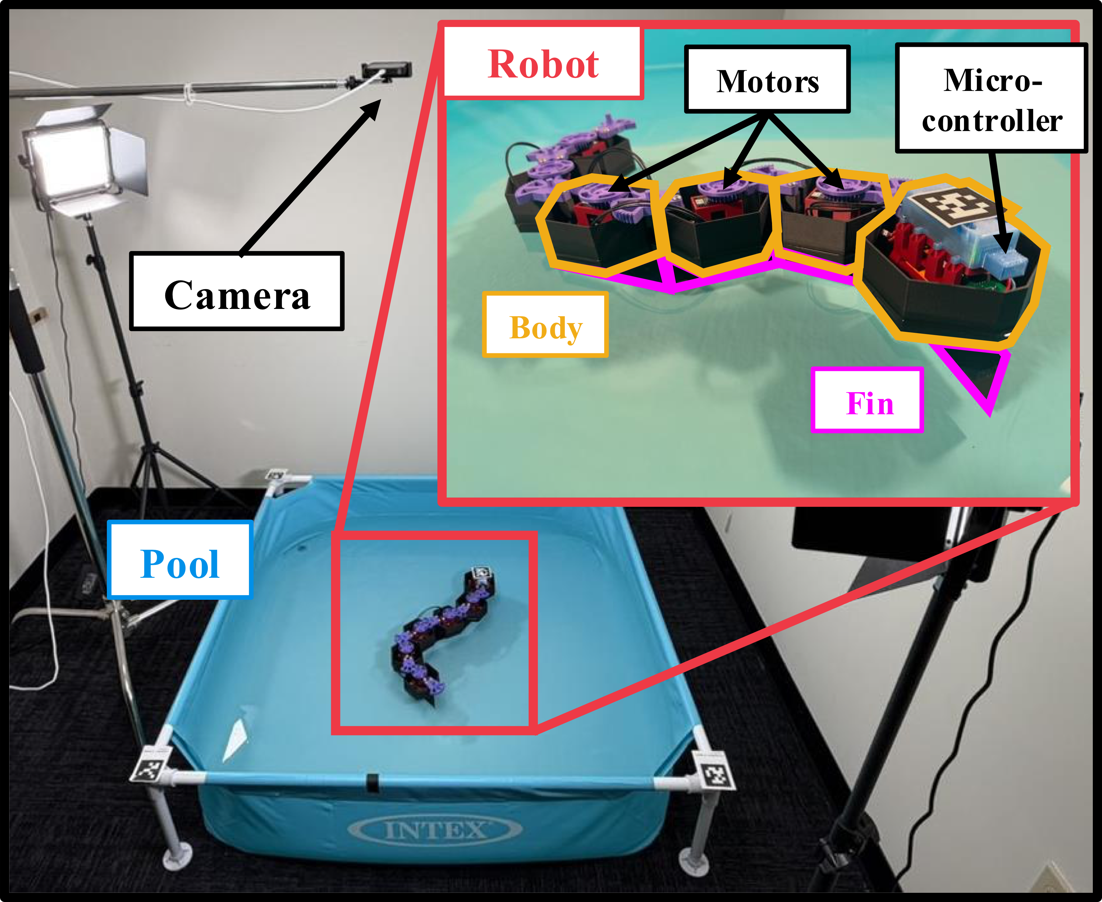
The eel robot has 6 rigid links (9.8 cm each) connected by revolute joints driven by Dynamixel XC330-M288-T servos. It is fully untethered, with an onboard 900 mAh battery and a Robotis OpenRB-150 microcontroller in the head link. Buoyant 3D-printed shells house the electronics; thin rigid fins underneath maintain a thin-plate hydrodynamic profile. Head-link pose is tracked by an overhead camera via AprilTags in a 122 × 122 cm pool, recreating the simulated walled cavity.

Hardware setup: a 122 x 122 cm pool with an overhead camera, and an inset showing the eel robot with annotated motors, body shells, fins, and microcontroller. — Sim-to-real validation setup. An overhead camera tracks AprilTags on the head link inside a 122 × 122 cm pool that recreates the simulated walled cavity. *Inset:* the bioinspired eel robot, with buoyant 3D-printed body shells housing the Dynamixel motors and head-link microcontroller; thin rigid fins underneath maintain a thin-plate hydrodynamic profile.

Bill of materials for SwimGym eel robot (2-link)
No.	Part Description	Material	Quantity	Price (USD)
1	3D-printing filament	PET-CF (3D printed)	1	$44.99
2	1-mm-thick plate	Fiberglass	1	$9.99
3	7.4V 900mAh LiPo battery	Lithium Polymer	1	$9.90
4	PCB board	FR-4 PCB	1	$3.00
5	25.4-cm-long JST wires	Wires	3	$1.41
5	EHR-3 connector	Plastic	2	$0.20
5	DC-to-DC Converters (OKR-T/6-W12-C)	Electronics	1	$9.24
6	OpenRB-150 MicroController	Electronics	1	$28.64
7	XC330/XL330-M288-T Servos	NA	1	$103.39 / $27.49
8	Fasteners (screws, helicoils, pins, etc.)	Stainless Steel	Multiple	$15.40
Total				$226.16 (Head) / $150.26 (Body)

Design

All design files can be found here.

Limitations and outlook

The experiments demonstrate substantially better sim-to-real fidelity than the particle-based baseline, but the model is not yet a complete description of the physical platform. The optimized C-start consistently undershoots the hardware travel distance, likely because the current model omits free-surface dynamics, servo compliance, detailed fin geometry, and uncertainty in mass properties and viscosity.

Computational scaling

Implicit integration is expensive, particularly in 3D. Future solvers must exploit sparsity and structure to scale to larger domains and longer-horizon optimization.

Representation tradeoff

The Eulerian grid is well suited to dynamic swimming and physical constraints, but is less convenient for visual rendering than particle-based fluid representations.

Beyond swimming

Promising extensions include implicit large-eddy simulation, design optimization, and other strongly coupled systems such as rigid-soft robots with contact.

05 · ResourcesCitation

@inproceedings{lee2026realizing,
  title     = {Realizing Robotic Swimming with Unified Fluid-Robot Multiphysics},
  author    = {Lee, Jeong Hun and Hu, Junzhe and Kwok, Sofia
               and Majidi, Carmel and Manchester, Zachary},
  booktitle = {Robotics: Science and Systems (RSS)},
  year      = {2026},
  note      = {Equal contribution: J. H. Lee and J. Hu}
}

06 · NotesAcknowledgments

The authors thank the members of the Robotic Exploration Lab and the Soft Machines Lab at Carnegie Mellon University for valuable discussions and feedback.

This work was supported by the National Science Foundation Graduate Research Fellowship under Grant No. DGE2140739.